Points3D - pointcloud modeling and registration software

QUICK START

1 REGISTRATION/ALIGNMENT

1.0 Alignment demo movie, automatic and manual registration

1.1 Automatic registration

After loading 3D files (see Loading pointclouds … ), click the registration tab on the left side of the main window. The top scans to register listbox displays all loaded scans. Adjust the number of neighbouring scans to check with the edit box below (how many neighbouring scans may have same overlapping surfaces? The number depends on your on-site scanning strategy. The smaller this number the faster the automatic registration will be).
The scan to scan listbox displays the scan pairs to check for alignment. Selecting individual scans in the top listbox with the usual CTRL, SHIFT keys will display these scans in the 3D-View and adjust the scan to scan checks – pairs.
Click the automatic registration  button to start the automatic alignment of the selected scans. The scans will be dealigned and a new alignment will be searched. The progress is shown in the progress bar and the memo at the bottom of the main window, see screenshot below. The alignment is divided into 4 jobs:

  • prepare, essentially indexing,
  • matching, first coarse matching,
  • i-check, first coarse verification,
  • adding, final best fit matching of found transformations and plausability checks.

The adding output line shows the overlap percentage of the 2 scans, the mean distance |dst| between the overlap ares, etc. or some error message in case of failure.

Successful matched scans are displayed in the 3D-View, failed scans are hided.

image 2: jobs and screenshot of memo output

memo2

1.2 Overlap statistics

To verify the quality of the alignment, click the overlap statistics button. The overlap statistics checks all visible scans for overlaps and calculates the mean distance |dst|, sigma, max/min and the overlap percentage. The distance calculation is done in that for each surface ray hittests are executed (reflects in hits and tested in the memo output). Each scan is divided into ground, ceilings, wallsA and wallsB surfaces and a separate statistic is presented for each of these groups. Main indicator for the precisement of the alignment is the overall mean distance |dst|.

image 3: overlap statistics output

Some words:

The registration is based on big data propabilistic analysis. Scans are divided into ceilings, grounds, walls A and perpendicular walls B. The scans should have overlap areas of ~5% with the A and B directions to succeed in automatic registration. Aligning 2 scans typically takes ~10 seconds. Within the test set (nearly 200 scans) the mean distance |dst| has been equal or better compared to target registrations.

1.3 Groups


Points3D starts aligning with the best matching scan pair and tries to fit the other scans to this first scan pair. This creates a first group of scans. If there are scans leftover not fitting into this group, a new group is opened with the next best matching scan pair-  and so on until all scans are assigned to a group or definitely are not assignable without breaking plausibility rules, i.e.failed. Subsequent transformations to a group member will be applied to all other members of the group, that is, manually aligning 2 groups requires only the matching of 2 scans.

The right popup of the top listbox offers possibilities to edit the groups:

  • undo/redo – last group action,
  • remove from group – to remove selected scans from a group,
  • new group – selected scans create a new group,
  • clear grouping – deletes all current groups,
  • show/hide group – shows/hides the group under the cursor.

1.3 Fine align all scans

The automatic registration  encompasses only a best fit matching between 2 scans. As a final step, click the fine align all scans (best fit)  button to carry out a best fit matching between all scans. In the example above (image 3), this leads to an improvement of the overall mean distance |dst| from 0.00284 m to 0.00203 m.

1.4 Manual registration

automatic registration  may not always succeed. To do a manual alignment, select the 2 scans to align i.e. in the scans to register listbox (hides all other scans in the 3D-View), then press the  manually registration button. Videos tell more than thousand words, so watch the following 3 movies to get a feeling for the manual alignment.

movie 1: manual registration basic

movie 2: manual registration - sewing technique

movie 3: manual registration - how to achieve something meaningful even with "failed" scans

Filtering in manual mode

As mentioned above, scans are divided into ground, ceiling, walls A and B elements. The task is to identify 3 corresponding walls A and B, ground or ceiling elements within the 2 scans. Aligning with mouseclicks means: element1/Scan1 is transformed to element1/Scan2 via the 2 mousclick-points and the element’s inherent normals. The transformation element2/Scan1 to element2/Scan2 is filtered in that only a perpendicular translation to the first transform is allowed, also the elements2 normal adjustment is limited to the perpendicular normal parts. The 3rd transformation is limited to only translate perpendicular to the first 2 transformations, no normal adjustment.
Tip and trick: holding down the SHIFT key moves an element only along it’s normal to the second element, the actual mouse click position is ignored in this case – similar to the 3rd transformation described above.

The filtering maybe reset with exiting and reentering the manual mode.
As the normal adjustment might imply some error, a sewing technique has been implemented (s. Movie 2): multiple clicks on one of the 3 direction elements are allowed and will lead to a rotation around the first clickpoint of this direction.

undo, redo, clear
all manual transformations are buffered and may be handled via those, hopefully, selfexplaining buttons.

1.5 2D registration image viewer

to view 2D images, click the small top right “show images” icon at the top of the scans to register listbox or right popup/“show scan images”. The viewer is intended for comparing scans, for orientation, identifying common parts and manually aligning scans. It shows the images of the first 2 selected scans. Selecting a new scan in the listbox will be displayed in the lower part.
  • Click the red up/down arrows icon to switch upper/lower image,
  • The red left/right icon switches between the original colors and the index-image, indices represented in false colors,
  • Red target icon to return to default autozoom center state,
  • Mouse wheel zooms in/out,
  • Right mouse button to pan an image,
  • Left mouse button to pan the whole viewer,
  • Mouse move shows the scan name and current index at the cursor in the bottom status bar,
  • Double click the top caption to enlarge/restore the image viewer,
  • Double click into an image selects a scan surface segment and depicts it in green.
  • see: 1.0 Automatic and manual registration demo movie to see how to use the viewer as a tool for manual registration.
The images are generated together with the .p3D files and are located in the \P3Ds\img subfolder.

1.5 Aligned scan pairs treeview

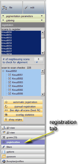
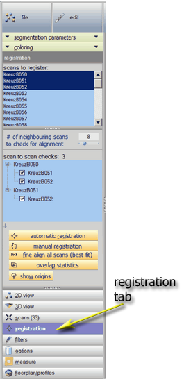
the treeview shows individual scanpairs. Directly matched pairs are displayed in black, not directly matched but both scans aligned in gray, error pairs in red. Use this treeview to check the correctness of the individual alignments. Use the left arrow button at the topright to toggle between this treeview and the scan to scan checks. Down button to inverse sorting of the pairs.

1.5 Alignment results

save all registered and visible scans via “file/export scans, meshes, points/visible scans to …” to pointcloud files *.ptx or CAD files *.obj for further workflowing. View a scan’s transformation matrix through righclick the scanitem in the scans to register listbox and select show transformation in the popup.

image 4: show transformation matrix

2 LOADING DATA

To load a pointcloud data file, click file/load 3d file(s).. and navigate i.e. to your FARO scans project directory to load *.fls scans (s. supported file formats). Loaded scans will automatically be meshed in the indicated range (segments) for auto-meshing: from/to index range. Selecting multiple scans results in parallel loading and will be automatically meshed as well.
The quality slider controls the quality of the triangulation (5 steps):

  • lowest quality 1: fastest, lowest number of vertices and points, easier to navigate in the 3D-View for a huge load of scans,
  • highest quality 5: takes more time, highest number of vertices and points.

The meshed scans will automatically be saved as .p3D files in the current scans sisterfolder \P3Ds thus allowing to quickly load the scans the next time needed (milliseconds as opposed to tens of seconds).

Loading a single scan, Points3D starts the segmentation process and displays the result in the 2D view in false colors for each identified surface. Doubleclicking on a segment or selecting one in the adjacent treeview will mark the selected segment in white. With the usual keys CTRL, SHIFT , multiple segments may be selected/deselected in the treeview as well as within the image. The treeview shows the segments sorted along their number of points (the indices), largest segment first. It also shows some basic features of a segment like its average Normal (N), area, 3D centerpoint (CP3D).

The segmentation result depends on three parameters adjustable within the segmentation parameters panel:

  • Distance threshold: neighbouring points exceeding this limit will not be included in the current segment,
  • Normals threshold: the normals of neighbouring points must be within this limit,
  • Lowpass normals window: the strength of the lowpass to adjust neighbouring normals.

The statusbar shows the current mouse position, the rgb pixel value, distance R and the xyz values. The scan image width/height/pixeldepth and the current zoomfactor(z) is shown to the right.

2D view popup Rightclick on the treeview or the scan image shows a popup menu with the options:

  • copy: copies the image to the clipboard,
  • autozoom: fits image to the 2D-viewer,
  • zoom 1.0: shows image 1:1,
  • save image: saves image to the \images\-subfolder of the programs current location,
  • switch image: toggles original and false color image,
  • selected pointclouds to 3D view to transfer the selected segments as pointclouds to the 3D view,
  • clear tree clears the treeview and frees the scan data.

3 THE 3D VIEW

3.1 Treeview panel

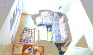
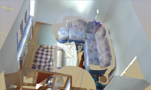
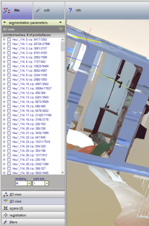
The 3D view shows a treeview on the left displaying the meshed surfaces. The treeview items show the scan’s filename first, limited to 8 characters (if the filename is longer, a ‘*’ is placed into the middle), followed by the surface’s sorting index, i.e. area. Appended is the number of triangle faces.
Subitems display some properties of the surface:

  • N, the normal,
  • area,
  • surrounding rectangle, which may be visualized when checked (displays as well N at CP3D and the convex hull),
  • number of faces and vertices,
  • the surface centerpoint CP3D.

Selected surfaces are shown in a turquoise color. For meshed surfaces the rendering dropdown offers different visualisations (fill, mesh, points – i.e. the vertex points). For pointclouds the size of the points maybe varied with the point size dropdown.

  •  

3.2  Mouse navigation

Within the 3D scene viewer:
  • Left mouse down: rotate the scene around the origin,
  • Mouse wheel: zoom in/out,
  • Mouse wheel + SHIFT: zoom in/out ten times slower,
  • Right mouse up: shows the 3DViewer popup,
  • Right/Middle mouse down + mouse move: pan the scene,
  • Left doubleclick: select the object (depicted turquoise) or deselect it,
  • Left doubleclick + SHIFT : hides the object,
  • Mouse move + CTRL: red sphere marks the intersection point of the camera-mouse-ray with a 3D-object (if one is found), the size of the sphere maybe adjusted with the pointing spheres radius slider on the options panel – also the scan’s name and index is displayed,
  • Left mouse down + CTRL: sets a polygon point for measuring (visualized with local dashed coordinate axes), values are shown on the status/ measure panel,
  • Mouse move + CTRL + SHIFT: starts measuring along a given direction (main axes x, y, z or a selected face normal) visualized with a dashed line, values are shown on the status/ measure panel,
  • Mouse move/down + CTRL + SHIFT: if the hullbox is visible and the mouse hint shows a hullbox plane, select the backward plane,
  • Mouse move + CTRL + ALT: shows and moves the profileplane along a selected normal, positive depicted white, negative black, movie 5 below,
  • Mouse move + CTRL + ALT + “y”: cuts the scene along the profileplane in dirty mode – releasing the “y“-Key cuts the scene clean, movie 6 below,
  • Mouse move + CTRL + “x“: for floorplan polylines, after hiding all objects, depicts the contributing walls, releasing CTRL hides the walls again (hit the “b” key to show them permanent), movie 7 below,
  • Right mouse down + ALT : pan selected mesh-objects,

3.3  3D View popup

Rightclick the treeview or the 3D Viewer to show its popup.

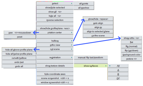
  • select all points: select all pointclouds transferred
    from the 2D View
  • select all meshes: all triangulated surfaces (to deselect all: click on the treeview where no item is present),
  • show/hide will also check/uncheck the corresponding treeview items,
  • show all, hide all, shortcut s key,
  • show/hide profileplane, shortcut esc key,
  • rotation center, shortcut r, to place a new pivot point,
  • hullbox
    • autoalign: aligns to the main axes of the scans,
    • align xy: aligns to the coordinate system,
    • align to selected plane,
    • cut the scene: cut off all parts outside the hullbox
  • ortho view
    • show ortho o, scans are displayed along the normal of the profileplane and aligned to the screen x/y,
    • flat: flattens all points to the ortho plane used,
    • flip (normal): flips the normal of the ortho plane, i.e front/back,
    • flip (up/down): 180° rotation,
    • background color: select a custom color,
    • restore r: return to last 3D state.
  • cut scene,
  • registration, items only enabled when registration tab is active.
    • flip last transform, in manual mode: invert last transformation,
    • show surfaces: show walls A/B, grounds and ceilings individually.
  • load textuture details: load and switch to textured mode
  • hide coordinate axes in case a screenshot without coordinates is needed
  • screenshot, 3D scene or whole window to clipboard, the image is also saved to the \images\-subfolder of the programs current location.

4 SCAN TAB

4.1 Scans treeview


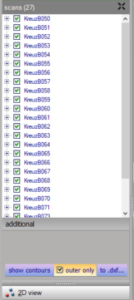
Multiple scans maybe loaded: “file/load 3D file..” and select multiple files. The loaded scans are displayed as items in the scans treeview. Checking/unchecking items shows/hides the scans in the 3D view. Selecting a scan item shows the scan in turquoise color. The subitem shows the number of all triangles for the scan. Use the treeview’s right popup to show/hide all/selected scans or remove selected scans. The additional panel allows to display the contour polylines of the visible surfaces. Individual faces may be selected with the show/hide feature of the Scans/3D-view treeview. The outer only checkbox filters inner (isles) contours. The shown polylines may be exported to a *.dxf file via the to .dxf  button.

5 FILTERS

5.0 Filter indices sliders

allows to limit the displayed faces to a certain range (indices are sorted along the faces areas).

5.1  Demirror

Use the demirror filter to remove annoying, unappealing mirrored parts of scans. For the automatic registration, those parts are not only unappealing, they can be real game stoppers for scans with many mirrors or glass fronts. Click the  demirror scans button to automatically demirror all visible scans. Edit and save the demirrored scans. See movie 4 below.  
movie 4: demirror a bathroom scan s. footnode[1]

5.2 Freehand select

freehand select faces and polylines with a lasso line, a great tool to quickly remove unwanted items from scans. To select: faces need to be entirely within the lasso line contour, polylines only to be touched. The freehand selection may at any time be activated with Alt + left mouse down, the cursor shows a + sign then.

Selected faces are displayed with a lime color, polylines as dashed lines. Use the hide/show button to display selections (if the button is down, newly selecteds will automatically hide).

Use deselect all to undo all selections.

Save the filtered scans with the “export scans, meshes, points/visible 3D meshes/points to ..” from the file main menu.

6 FLOORPLAN/PROFILES

6.1  Profileplane

To show and move the profileplane, hold down the CTRL + ALT keys and move the mouse. The profileplane has the properties base position (base pos.), i.e. where it was originally positioned and its normal. Moving the plane shows a white/black line starting from the base position along the plane’s ± normal’s direction ( see: movie 5 below).The actual distance from the base position is shown with the dst-slider.

The default profileplane has a normal in z-direction and base pos. z = 0. To define another profileplane, mouseclick + CTRL a surface of interest. This sets the base position at the marked point and the normal along the marked surface’s normal.


Move the alpha and theta sliders to rotate the profileplane around its 2 intrinsic axes. Adjust the profileplane transparency with the corresponding slider.

The cursor key changes edit allows to set the moving step when using when using the left/right/up/down cursor keys. The left/righ cursor keys move the profile plane, the up/down keys also cut the scene.

movie 5: defining and moving the profileplanes. footnode[1]

6.2  Cutting a scene with the profileplane

Watch movie 6 below to see the scene cutting technique. Instead of the combination CTRL + ALT + y + mousemove you may use the up/down arrow keyboard keys to move through the scene, as long as the profileplane is visible.

movie 6: cutting a scene with the profileplan s. footnode[1]

6.3    Floorplan

Click the floorplan with visible meshes-button to automaticaly create a floorplan of the visible scene. For the auto-floorplan, the mass-center-point (CP3D) of a heuristic determined ground surface is taken for the base position of the projection plane, the projection plane’s normal is the z-axis. All wall surfaces with a normal lying in the range 90° ± 30° to the z-Axis will be taken for the floorplan projection.
Only contour points of those walls will be projected. To avoid ambiguous projection lines, the lower contour points are considered only.
Limit the range of contour points with the projection limit-slider in [m], i.e. limit points to a distance less than the sliderposition. The cut limits-button shows these projection limits.

Use the hide-button to hide/show the profileplane and the floorplan polyline, the clear-button clears the polyline buffer. Use to .dxf… to export the floorplan polylines to a .dxf file.
movie 7: floorplan s. footnode[1]

6.4  Single profile

Move the profileplane to a location where you want to take a profile of the visible scene,
i.e. a cut of the profileplane with the scene. Check extrapolate for edge hits within the right drop-out pane to extrapolate the profile-polylines – this is for easier detection of corners (see animation below).

The right drop-out pane offers editing some properties of the profile lines. Check “move lines with profile plane” to place the lines at a more convenient point (i.e. use the profiles for a floorplan without skirting boards). The “connect lines” button automatically connects close lines.

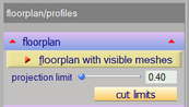
6.5  Autocreate profile series

Place the profileplane as described above, move it with CTRL + ALT + mousemove and watch the dst-slider to find the range. Edit the from, to and step values accordingly, click start. Points3D will generate a series of profilelines separated by the step value. The limit angle-slider filters out surfaces with an angle (surface.normal vs. profileplane.normal) smaller than that value. The slider controls level/contour lines of parallel surfaces. Setting it to zero allows to depict irregularities of surfaces.  see movie 8 below. Check single profile/right drop-out pane/extrapolate for edge hits to extrapolate the polylines for edges. After creating a profile series, you may check/uncheck the project profilelines-box to project all lines onto the profileplane and back again. Export the lines with the “to .dxf… -button.

 
movie 8: high resolution profile series s. footnode[1]

6.6    Gridbox

gridbox searches for the main axes of the scene. It then generates profiles in the corresponding x’, y’, z’ directions with the step value from the autocreate profile series panel. Again, check single profile/right drop-out pane/extrapolate for edge hits to extrapolate the polylines for edges

7 OPTIONS

7.1 Options panel

general tab

The options tab allows to change the 3D Viewer background colors, select predefined views. The maximum history of recent opened files as displayed in the main menu’s file/recent list may be editet here.

Check threads: load fls-scans as ext. jobs to load multiple pointcloud-files (fls, ptx) parallel with external threads. The number of external threads is currently limited to half of the available CPU-processors, a “waiting for:…” message in the mainwindow’s bottom memo shows the progress.

Check save processed files to ..\P3D\*.p3d to dump pointcloud-files as p3d-files into a sibling folder. Loading .p3d-files might speed up loading by a factor of 100 and more.

Check show absolute coordinates to show and export all coordinates in absolute coordinate values of your scan-project – if available. Note: the origin of the 3D view coordinate system is placed into the origin of the first scan opened – the masterscan.

Adjust the pivot sphere radius to mark the current rotation center,  the pointing sphere radius displayed at the mouse position, screenshot dpi resolution and the mouse wheel zoom factor to adjust wheeling zoom behavior (s. Mouse navigation above).


color tab:

the coloring dropdown offers the following coloring schemes:

  • false colors,
  • normals (directions as color values),
  • distance gray (distances as gray values),
  • original colors.

8 MEASURE

8.1 Measurement

Points3D offers some basic 3D measurement. Follow the instructions 
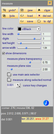
on the measure tab to start 3D measuring. The gray display shows in the first row the last intersected mesh object and the mouse values, in the 2nd row the xyz values of the last mouse intersection point and the angle to the last selected object’s normal, in the 3rd row the distance from the last marked polygon point (blue sphere) to the last mouse intersection point (red sphere), and, on the buttonstyle pane, the overall polygon length. The 4th row finally shows the distance along the normal (when holding down the CTRL + SHIFT keys) and any hit distances with other mesh objects – see movie 9 below. These values are also reflected on the status bar. The size of the pointing spheres and polygon nodes maybe adjusted with the pointing spheres radius- slider. The undo-button removes the last polygon node. Press the clear-button to clear the measurement.
movie 9: measurements

9 MODELING

The model tab offers:

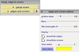
  • merge scans: merges the overlaps (duplicates) of all visible scans giving a more homgenous presentation and reducing the number of triangles by the overlap factors. For best accuracy, triangles discarded are determined by their distance to the scan origins. Having no doublettes certainly makes measurements more easy and preciser.
  • edges and corners: automatically detect edges and corners of visible scans. It creates a gridbox and expands the gridbox lines for intersections. Set the grid box steps within the right drop-out pane, where also some properties of the result may be edited.

10 TEXTURE, RESOLUTION & CULLING

In the lower right status panel there are 3 circle symbols. Click:

  • blue/green: switch between high and low resolution, i.e high/low number of triangles. Low resolution usually has a couple of 100 times less triangles. This mode is extremely useful if you loaded many scans and the graphic card gets down and hinders navigation.
  • purple/red: switch culling on/off in low resolution mode. Culling means faces overlapped by other faces on the camera axes will be removed from the rendering pipe. This also speeds up navigation.
  • turquoise/yellow: load and switch textured mode. Texture mode improves the realistic look and feel, s. the animation below.

11 SUPPORTED FILE FORMATS

11.1    Read files

.fls Fls-file, FARO laser scan file format
.p3d p3d-file, Points3D fast and compact internal format for meshed objects
.ptx ptx-file, Leica plain text data format (PTX)
.asc ASCII text format for 3D pointcloud
Note: For asc – files, the data is expected in the following order per line: x, y, z, I (I for Intensity, is optional)
.xyz XYZ text format for 3D pointcloud, as exported i.e. by Faro scene
Note: For xyz – files, the data is expected in the following order per line: u,v (pixel values), x, y, z, r, g, b
.obj WaveFront model file
.stl Stereolithography file

11.2    Write files

.p3d p3d-file, Points3D fast and compact internal format for meshed objects
.ptx ptx-file, Leica plain text data format (PTX)
.obj WaveFront model file for meshed objects
.stl Stereolithography file
.dxf Autodesk Drawing Interchange File Format (polylines and triangles)
.xyz XYZ text format for 3D pointcloud

12 SYSTEM REQUIREMENTS

12.1 Minimum configuration

Points3D is 64bit and therefore windows 64bit is mandatory.

  • Microsoft Windows 7/10/11,
  • Intel i7 and up,
  • 16 GB,
  • Mid range graphics card,
  • OpenGL 4.4 and higher.

FOOTNOTES

[1] = movie was created with version 4.00, GUI changed, the shown functionality not.